Use the empirical rule calculator to find 68-95-99.7 normal-distribution bands, exact probabilities, tail areas, z-score context, and Chebyshev bounds.
Last updated
Empirical rule calculator for the 68-95-99.7 normal distribution rule Enter a mean, standard deviation, and optional observed value to see the exact 1σ, 2σ, and 3σ bands, tail areas, section probabilities, z-score, percentile, and Chebyshev comparison for the same distribution.
Examples
Normal-model assumption
The empirical rule applies to approximately bell-shaped, symmetric data. Use the Chebyshev rows when you need a conservative comparison for data that may not be normal.
Result
68.27% within 85 to 115
For μ = 100 and σ = 15, the calculator reports exact normal-CDF probabilities behind the rounded 68-95-99.7 rule.
68.27%
Within 1σ
95.45%
Within 2σ
99.73%
Within 3σ
1
Observed z-score
84.13%
Percentile
Inside ±1σ
Observed band
Observed value: Inside ±1σ This value is in the central empirical-rule band, so it is typical under a normal model.
84.13% of the normal model lies at or below x = 115, 15.87% lies above it, and the two-tailed extremeness is 31.73%.
Empirical-rule bands
Exact normal probabilities are shown beside the rounded classroom rule and the remaining tail area.
Band
Range
Exact probability
Outside total
Each tail
μ ± 1σ
85 to 115
68.27%
31.73%
15.87%
μ ± 2σ
70 to 130
95.45%
4.55%
2.28%
μ ± 3σ
55 to 145
99.73%
0.27%
0.13%
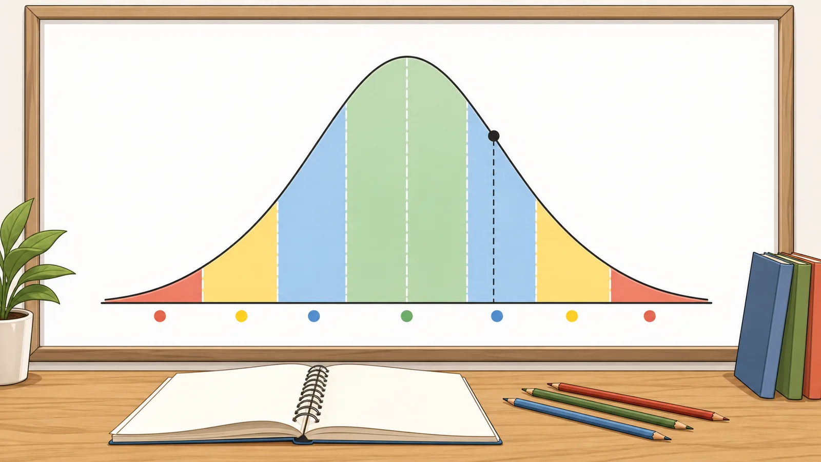
Section probability breakdown
These rows split the bell curve into the same regions often shown in empirical-rule diagrams.
Below −3σ: Below 55
Extreme low tail beyond the empirical-rule range.
0.13%
−3σ to −2σ: 55 to 70
Low outer band; unusual but still inside ±3σ.
2.14%
−2σ to −1σ: 70 to 85
Low shoulder between the 68% and 95% bands.
13.59%
−1σ to mean: 85 to 100
Lower half of the central 68% band.
34.13%
Mean to +1σ: 100 to 115
Upper half of the central 68% band.
34.13%
+1σ to +2σ: 115 to 130
High shoulder between the 68% and 95% bands.
13.59%
+2σ to +3σ: 130 to 145
High outer band; unusual but still inside ±3σ.
2.14%
Above +3σ: Above 145
Extreme high tail beyond the empirical-rule range.
0.13%
Empirical rule vs Chebyshev
Chebyshev's inequality is weaker but works for any distribution with a finite standard deviation.
Empirical rule calculator: 68-95-99.7 rule, sigma bands, and normal-model tails
The empirical rule calculator applies the 68-95-99.7 rule to a normal distribution, then shows the exact probability, raw-score range, outside-tail area, and observed-value interpretation for the mean and standard deviation you enter.
What this empirical rule calculator covers
This page computes the three classic empirical-rule bands: μ ± 1σ, μ ± 2σ, and μ ± 3σ. It returns the rounded classroom rule values of 68%, 95%, and 99.7% alongside the exact standard normal probabilities of about 68.27%, 95.45%, and 99.73%.
Competitor pages often stop at the three interval ranges. This calculator also shows the outside area, each tail, a section-by-section bell curve breakdown, an observed-value z-score and percentile, and a Chebyshev comparison so you can see what changes when the normal-distribution assumption is weakened.
Use the observed value field when the question is not only "what are the 68-95-99.7 ranges?" but also "where does this specific score or measurement fall?" The result classifies the value as central, unusual, or beyond the usual empirical-rule range under the normal model.
The 68-95-99.7 rule
The empirical rule states that for an approximately normal distribution, about 68% of values lie within one standard deviation of the mean, about 95% lie within two standard deviations, and about 99.7% lie within three standard deviations.
The rounded figures are easy to remember, but the exact values come from the standard normal cumulative distribution function. This calculator uses the exact CDF probabilities while still showing the familiar rule-of-thumb meaning.
For example, if a normal model has μ = 100 and σ = 15, then the one-sigma band runs from 85 to 115, the two-sigma band runs from 70 to 130, and the three-sigma band runs from 55 to 145.
P(μ − kσ < X < μ + kσ) = Φ(k) − Φ(−k) = 2Φ(k) − 1
Probability within k standard deviations, where Φ is the standard normal cumulative distribution function.
Range = μ ± kσ
The raw-score interval for k = 1, 2, or 3 standard deviations from the mean.
How the section probability breakdown works
A full empirical-rule diagram is more detailed than the three headline percentages. The middle band from the mean to +1σ contains about 34.13% of the normal curve, and the matching band from −1σ to the mean contains the same amount. The shoulders between 1σ and 2σ contain about 13.59% on each side, and the outer bands between 2σ and 3σ contain about 2.14% on each side.
The remaining area beyond ±3σ is small but not zero. Under a perfect normal model, each tail beyond three standard deviations contains about 0.135% of the distribution. That is why values past 3σ are often treated as extreme, but they are still possible in large samples.
Observed value, z-score, percentile, and tails
The observed value field converts a score or measurement into a z-score using z = (x − μ) / σ. A value at z = 0 is exactly at the mean. A value at z = 1 is one standard deviation above the mean. A value at z = −2 is two standard deviations below the mean.
Once the z-score is known, the calculator reports the normal-model percentile, the area above the value, and the two-tailed extremeness. This makes the empirical rule more useful for real questions such as whether a test score is typical, whether a measurement is unusual, or whether a process value is far enough from the mean to investigate.
z = (x − μ) / σ
Standardise an observed value by measuring its distance from the mean in standard-deviation units.
Percentile = Φ(z) × 100
The normal-model share of values at or below the observed value.
Empirical rule versus Chebyshev's inequality
The empirical rule is powerful because it gives tight percentages, but it depends on an approximately normal, bell-shaped distribution. Chebyshev's inequality is weaker but applies to any distribution with a finite mean and standard deviation.
For k greater than 1, Chebyshev guarantees that at least 1 − 1/k² of the distribution lies within k standard deviations of the mean. At 2σ, that lower bound is 75%, compared with about 95.45% for a normal distribution. At 3σ, Chebyshev gives at least 88.89%, compared with about 99.73% for a normal distribution.
The comparison table is a caution tool. If your histogram is clearly skewed, multimodal, bounded, or heavy-tailed, the empirical rule may overstate how much data is inside the middle bands.
Chebyshev minimum within kσ = 1 − 1/k², for k > 1
Distribution-free lower bound for data within k standard deviations of the mean.
When to use the empirical rule
The empirical rule is best for quick interpretation when the data are roughly symmetric, bell-shaped, and unimodal. It is common in introductory statistics, measurement-error intuition, test-score examples, and quality-control conversations where a normal model is a reasonable approximation.
It should not be used as a blind rule for heavily skewed data, multimodal data, bounded data, or data with many outliers. Always check the data shape with a histogram, density plot, normal probability plot, or domain knowledge before treating the 68-95-99.7 bands as meaningful probabilities.
Worked example: IQ-style scale
Suppose a normally distributed scale has μ = 100 and σ = 15. The 1σ band is 85 to 115, and about 68.27% of values fall inside that range. The 2σ band is 70 to 130, and about 95.45% fall inside it. The 3σ band is 55 to 145, and about 99.73% fall inside it.
If an observed value is x = 130, then z = (130 − 100) / 15 = 2. The normal-model percentile is about 97.72%, meaning about 2.28% of values lie above that score. The value is unusual but still inside the 3σ empirical-rule range.
What this calculator does not prove
This calculator does not test whether a dataset is normal. It does not estimate the mean or standard deviation from raw data, and it does not replace a normality test, residual check, or domain-specific model review.
It also does not prove that a value is an error. A point beyond 3σ can be a data-entry mistake, a real but rare observation, a sign that the model is wrong, or evidence that the process changed. Treat the result as a normal-model interpretation, then verify it against the actual data and context.
Frequently asked questions
Is the empirical rule exact?
The rounded 68%, 95%, and 99.7% figures are approximations. The exact normal-CDF values are about 68.27%, 95.45%, and 99.73%. This calculator reports the exact values while keeping the familiar rule labels easy to recognise.
Does the empirical rule apply to all data?
No. It applies to data that is approximately normally distributed. If the data are skewed, bimodal, heavy-tailed, strongly bounded, or full of outliers, the empirical-rule percentages can be misleading.
What is the difference between the empirical rule and Chebyshev's inequality?
The empirical rule gives tight percentages but assumes a normal distribution. Chebyshev's inequality gives weaker minimum guarantees but works for any distribution with a finite mean and standard deviation. At 2σ, Chebyshev guarantees at least 75%, while a normal distribution has about 95.45% inside that range.
How do I find the range for 95% of normally distributed data?
Use μ ± 2σ. Subtract two standard deviations from the mean for the lower bound and add two standard deviations for the upper bound. Under a normal model, the exact probability inside that range is about 95.45%, often rounded to 95%.
How much data is outside three standard deviations?
Under a normal distribution, about 0.27% of values are outside ±3σ in total. That is about 0.135% in each tail. Those values are rare, but they are not impossible, especially in large datasets.
What does an observed z-score tell me?
A z-score tells you how many standard deviations an observed value is from the mean. Positive z-scores are above the mean, negative z-scores are below it, and larger absolute values are more unusual under the normal model.
Can I use this calculator to check for outliers?
It can flag values that are unusual under a normal model, especially values beyond 2σ or 3σ, but it cannot prove that a value is an outlier. Use it with plots, context, sample size, measurement knowledge, and a more formal outlier method when the decision matters.
Why does the standard deviation have to be greater than zero?
The standard deviation measures spread. If σ is zero, every value is identical and the z-score formula divides by zero. The empirical-rule bands collapse to one point, so the normal-spread interpretation no longer works.
Can I use the empirical rule with sample mean and sample standard deviation?
You can use sample statistics as an approximation when the sample is large and representative, but the result is model-based. For small samples or uncertain distributions, inspect the data shape and treat the bands as estimates rather than guarantees.
How is this different from a normal distribution calculator?
A normal distribution calculator can answer many tail, interval, percentile, and inverse-normal questions for any cutoff. This empirical rule calculator focuses on the memorable 1σ, 2σ, and 3σ bands, plus the observed-value context needed to interpret those bands quickly.