Use this normal distribution calculator to find left-tail, right-tail, two-tailed, and between-two-values probability for any bell curve.
Last updated
Normal distribution calculator for left-tail, right-tail, interval, percentile, and z-score questions Use one bell curve model to answer the probability below a score, the probability above a score, the probability between two values, or the raw cutoff behind a percentile. The result sheet keeps percentile rank, tail area, and benchmark ranges in view so the answer is useful after one interaction.
Solve mode
Find a left-tail, right-tail, or two-tailed probability for one cutoff.
Tail selection
Quick examples
Result
95%
P(X ≤ x). 95.00% of the distribution lies at or below 1.645, which is 1.65 standard deviations from the mean.
95%
P(X ≤ x)
95%
P(X ≤ x)
5%
P(X ≥ x)
10%
Two-tailed area
1.65
Z-score
95th
Percentile rank
1.645 sits 1.65 standard deviations above the mean, so about 95.00% of outcomes fall at or below that point. For a continuous bell curve, probabilities come from areas to the left, right, or between bounds. A single exact point has zero probability mass, which is why normal distribution questions are usually framed as tail or interval areas.
Mean (μ)
0
Standard deviation (σ)
1
Value (x)
1.65
Z-score
1.65
Percentile rank
95th
P(X ≤ x)
95%
P(X ≥ x)
5%
Two-tailed area
10%
Empirical-rule checkpoints
These rows answer a common follow-up question: what raw-score ranges correspond to the classic 68–95–99.7 coverage bands for this same normal distribution?
Band
Lower value
Upper value
Coverage
Within 1σ
-1
1
68.27%
Within 2σ
-2
2
95.45%
Within 3σ
-3
3
99.73%
Percentile cutoffs in the same distribution
Use this table when the next question is the reverse one: which raw score marks the 90th percentile, 95th percentile, or another common bell curve cutoff if the same mean and standard deviation stay in force?
Normal distribution calculator — bell curve probability, percentile, and interval guide
A normal distribution calculator helps you answer several different bell curve questions with the same mean and standard deviation: the probability below a value, the probability above a value, the probability between two values, the percentile rank of a score, or the raw cutoff that matches a target percentile.
What this normal distribution calculator covers
This page now handles the main search intents that appear across competitor pages: left-tail probability P(X ≤ x), right-tail probability P(X ≥ x), two-tailed extremeness, probability between two values, percentile-to-value conversion, and z-score-to-value conversion. That matters because a good normal distribution probability calculator should not force you to bounce between several separate tools just to answer closely related bell curve questions.
If you already know the mean and standard deviation, you can use the same calculator to move between raw scores, z-scores, percentile cutoffs, and interval probabilities. The result sheet is designed to keep those views connected so the output stays useful for teaching, quality-control checks, test-score interpretation, and threshold planning.
The normal distribution and the bell curve
A normal distribution is fully described by two parameters: the mean μ, which sets the centre of the distribution, and the standard deviation σ, which sets the spread. The curve is symmetric and bell-shaped, so values near the mean are common while values far from the mean become progressively rarer.
Many introductory statistics questions use the normal curve because it is mathematically tractable and often a reasonable model for measurement error, biological traits, exam scores, and averages of many small effects. The empirical rule is the quick summary: about 68% of values fall within one standard deviation of the mean, about 95% within two, and about 99.7% within three.
Mean, standard deviation, and what they control
The mean μ tells you where the distribution is centred. If μ = 100, the curve is balanced around 100. The standard deviation σ tells you how wide the curve is. A small σ means values cluster tightly around the mean, while a large σ spreads the same total probability across a wider range of raw scores.
Those two inputs are the reason the same percentile or z-score can map to very different raw values in different settings. A 95th percentile cutoff on a narrow distribution may sit only a little above the mean, while the same percentile on a wider distribution can be much further away in the original units.
Probability below, probability above, and why a point itself has zero probability
For a continuous distribution such as the normal distribution, probability is represented by area under the curve. That is why normal-distribution questions are usually written as P(X ≤ x), P(X ≥ x), or P(a ≤ X ≤ b). The area to the left of x is the cumulative distribution function, often written Φ(z) after converting the raw score to a z-score.
This also explains a common point of confusion: the exact probability of one single point on a continuous curve is zero. In practice, a normal distribution calculator reports the probability below a cutoff, above a cutoff, or between two cutoffs. Those are areas, not point masses.
Z-score and standardisation
To find the probability for any normal distribution, convert the raw value x to a z-score using z = (x − μ) / σ. The z-score measures how many standard deviations the value sits above or below the mean. Once the value is expressed on the standard normal scale, the same cumulative distribution function can be reused for any bell curve.
For example, if μ = 100 and σ = 15, then x = 115 gives z = 1. That means the score is one standard deviation above the mean, which corresponds to about the 84th percentile. Converting to z first is why a normal curve calculator can move cleanly between raw scores, tail areas, and percentiles.
How to find the probability between two values
A major reason people search for a normal probability calculator is to answer interval questions such as the probability between 85 and 115, the share of parts inside tolerance, or the percentage of scores inside a planning band. The calculation is straightforward once both endpoints are standardised.
If a is the lower bound and b is the upper bound, convert both to z-scores and subtract the two cumulative probabilities: P(a ≤ X ≤ b) = Φ(z_b) − Φ(z_a). This page now handles that interval workflow directly instead of making you run two separate left-tail calculations and combine them manually.
P(a ≤ X ≤ b) = Φ((b − μ) / σ) − Φ((a − μ) / σ)
Interval probability is the difference between the cumulative probabilities at the upper and lower bounds.
One-tailed versus two-tailed interpretation
A left-tail probability asks how much of the distribution lies at or below a value. A right-tail probability asks how much lies at or above it. A two-tailed interpretation asks a different question: how much of the distribution is at least this far from the mean in either direction?
That distinction matters because the same raw score can sound very different depending on the question. A point 1.96 standard deviations above the mean leaves about 2.5% in the upper tail, but about 5% in the two tails combined. If you are thinking about extremeness, screening cutoffs, or hypothesis-testing intuition, the two-tailed area is often the more relevant framing.
Percentiles, quantiles, and inverse normal cutoffs
Sometimes the question is reversed. Instead of asking for the probability below a score, you want the score that marks the 90th percentile, 95th percentile, or another quantile. In that case, the calculator works backward from the cumulative probability to the matching z-score and then converts that z-score back to the original scale.
This is the workflow behind search phrases like normal distribution percentile calculator, inverse normal calculator, or value from percentile. It is useful for exam cutoffs, staffing thresholds, service-level targets, and any planning decision that starts with a percentile goal rather than an existing raw score.
z = (x − μ) / σ
Standardise a raw score to the standard normal scale.
P(X ≤ x) = Φ(z)
Left-tail cumulative probability for the corresponding z-score.
x = μ + zσ
Convert a z-score or percentile cutoff back to the original scale.
Empirical-rule checkpoints in raw-score terms
The 68-95-99.7 rule is easiest to remember on the z-scale, but most real users think in the original units. If the mean is 100 and the standard deviation is 15, then the middle 68% sits roughly between 85 and 115, the middle 95% between 70 and 130, and the middle 99.7% between 55 and 145.
Displaying those raw-score bands makes the spread of the distribution easier to explain to non-specialists. It also helps when the next question is operational rather than academic: which values look typical, which are clearly unusual, and which are extreme enough to trigger review?
Worked examples
Suppose test scores are normally distributed with μ = 100 and σ = 15. For x = 120, the z-score is (120 − 100) / 15 ≈ 1.33. The left-tail probability is about 90.9%, meaning roughly 90.9% of scores fall at or below 120 and about 9.1% lie above it.
For an interval example, the probability between 85 and 115 is the classic one-standard-deviation band around the mean. That interval contains about 68.3% of the distribution. For a percentile example, the 95th percentile cutoff is about x = 100 + 1.645 × 15 ≈ 124.7.
When a normal model is useful and when it is not
A normal model is often reasonable for smooth, roughly symmetric, unimodal data, especially when the variable is continuous and not strongly bounded. It is also common as an approximation for averages because of the central limit theorem.
The model becomes less trustworthy when the data are strongly skewed, heavily tailed, multimodal, bounded near a hard floor or ceiling, or clearly discrete. In those cases, a bell curve calculator can still be useful for rough intuition, but the percentile and tail probabilities should be treated as model-based approximations rather than direct facts about the observed dataset.
Common applications
Quality control uses the normal distribution to translate tolerance bands into defect risk. Exam interpretation uses the same framework to convert a raw score into percentile rank or to set a percentile-based cutoff. Operations teams use bell curve thresholds to estimate how often service times, measurements, or demand levels will exceed a target.
In formal statistics, the standard normal curve also underpins z-tests, confidence intervals, and many textbook probability examples. That is why a strong normal distribution calculator should connect raw values, z-scores, percentiles, tails, and interval areas instead of treating them as unrelated tasks.
Frequently asked questions
How do I use a normal distribution calculator for probability between two values?
Enter the mean and standard deviation, switch to the interval workflow, and provide the lower and upper bounds. The calculator converts both bounds to z-scores and subtracts the two cumulative probabilities to get the area between them. This is the standard way to answer bell curve questions about a range rather than a single cutoff.
What is the difference between left-tail, right-tail, and two-tailed probability?
Left-tail probability is the share of the distribution at or below a value. Right-tail probability is the share at or above that value. Two-tailed probability combines both extremes and asks how much of the distribution lies at least as far from the mean in either direction. The correct choice depends on the actual question you are trying to answer.
How do I find the 95th percentile of a normal distribution?
The 95th percentile corresponds to a z-score of about 1.645 for a one-sided cumulative lookup. Convert that z-score back to the original scale with x = μ + zσ. For example, if μ = 100 and σ = 15, the 95th percentile is about 124.7.
What does the standard deviation tell me about the distribution?
A larger standard deviation means the bell curve is wider and values are more spread out around the mean. A smaller standard deviation means values cluster more tightly around the center. The same percentile cutoff moves further away from the mean when the standard deviation is larger.
Why is the standard normal distribution (μ = 0, σ = 1) special?
Any normal distribution can be converted to the standard normal by using z = (x − μ) / σ. That lets one cumulative distribution function handle every bell curve after standardisation. It is the shared reference scale for z-scores, percentile conversion, and tail-area interpretation.
What is the 68-95-99.7 rule?
For an approximately normal distribution, about 68% of values fall within one standard deviation of the mean, about 95% within two, and about 99.7% within three. It is a fast way to estimate how much of the bell curve lies in the middle versus the tails.
Can I use a bell curve calculator for percentile rank?
Yes. If you enter a raw score together with the mean and standard deviation, the calculator can convert that value into a z-score and then into a percentile rank under the normal model. That percentile is model-based, so it works best when the underlying data are reasonably close to normal.
What if my data is not normally distributed?
The normal distribution is a model, not a guarantee. If the data are strongly skewed, heavily tailed, bounded, or multimodal, the resulting percentiles and tail probabilities may be misleading. In that situation, check the data shape directly with plots or use a distribution that better matches the process.
Why must the standard deviation be greater than zero?
If the standard deviation is zero, every value is identical and there is no spread to measure. The z-score formula divides by the standard deviation, so a zero spread makes the standardized position undefined. Without spread, percentile and tail-area questions on a bell curve no longer make sense.
Is this the same as a z-score calculator?
The workflows overlap, but they are not identical. A z-score calculator focuses on standardised distance from the mean, while a normal distribution calculator also answers interval probability, percentile cutoff, and one-tail versus two-tail questions. This page includes z-score conversion as one part of a broader bell curve toolkit.